DetectiV: Analysis of pathogen detection microarray data

• Introduction
• Availability
• Installation
• Tutorial
• Supporting Data
• Author

Tutorial

This document is a tutorial for the DetectiV software. The tutorial contains code that can be directly executed in R, the software on which DetectiV is based.

• 1. Requirements
• 2. Getting some data
• 3. Visualisation 1
• 4. Normalisation
• 5. Significance Testing
• 6. References

1. Requirements

You will need:

• i) R, from http://www.r-project.org
• ii) the latest version of DetectiV, available from Sourceforge
• iii) the limma package, available from Bioconductor
• iv) the GEOquery package, available from Bioconductor

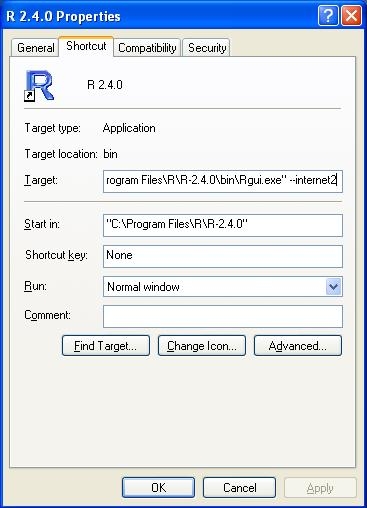
Connecting R to the internet

If you're having problems with R accessing the internet, then there are a couple of things to try.

On windows, right click the shortcut to R, and click properties. In the target box, enter the flag '--internet2':

On linux or unix systems, if you are using a proxy server, make sure your http_proxy environment variable is set and you may also need to 'unset no_proxy'.

2. Getting some data

Using the data already in the package

Using GEOquery

Code for retrieving data from GEO can be found in the /doc folder of the DetectiV package, however if you want to do it yourself, here is an example:

library(GEOquery)

gse2228 <- getGEO("GSE2228")
gsmplatforms <- lapply(GSMList(gse2228), function(x) {
 Meta(x)$platform
 })
probesets <- Table(GPLList(gse2228)[[1]])$ID
gse2228.matrix <- do.call("cbind", lapply(GSMList(gse2228), function(x) {
 tab <- Table(x)
 mymatch <- match(probesets, tab$ID_REF)

 return(tab$CH1_MEDIAN[mymatch])
}))

gse2228.matrix[is.na(gse2228.matrix)] <- 0
gse2228.matrix[gse2228.matrix<=0] <- 0.5

# get the genes

gse2228.genes <- Table(gse2228@gpls[[1]])

Alternatively, at time of writing the data can be downloaded as files:
GSE2228
GSE546

and then loaded using GEOquery:

library(GEOquery)
gse2228 <- getGEO(filename="GSE2228_family.soft.gz")
gse546  <- getGEO(filename="GSE546_family.soft.gz")

Using limma

Limma is a package from bioconductor for the analysis of microarray data. It contains functions to read in microarray data from many common formats. Here is an example of using limma to read in some genepix files (not provided):

# load the library

library(limma)

# find your gpr files
# NB: substitute your own value for the directory

setwd("C://path//to//a//directory//containing//gprfiles")
myfiles <- dir(pattern="gpr")
RG <- read.maimages(myfiles, source="genepix")

Preparing the data

Before we visualise the data, we need to prepare the data. This includes averaging over replicate probes and joining the data to probe annotation data. If you used the data(DetectiV) command, then the probe annotation data for the Urisman et al dataset will already be loaded:

data(DetectiV)
?grouping
grouping[1:10,]

However, if you did not use the data(DetectiV) command, you must load the probe annotation information. There is a file, "oligo_annotation.txt" in the /doc folder of the DetectiV package. This can be loaded:

grouping <- read.table(file="oligo_annotation.txt",
                       header=TRUE, sep="\t", quote="")

grouping[1:10,]

The next stage is to prepare the data by joining the intensity information to the probe annotation and averaging over replicate probes (where appropriate):

# we give the prepare.data() function:
#      - the matrix of intensities, with rows representing probes and columns arrays
#      - a vector of probe identifiers, one per row of the above matrix
#      - a data frame of data representing probe annotation
#      - the name of the column within the probe annotation that contains the probe identifiers

# for GEOquery data

gse2228 <- prepare.data(gse2228.matrix, gse2228.genes$OLIGO_ID, grouping, "UID")

# For limma data (presuming intensities are in the Cy3 channel)
# Background corrected:

gdata <- prepare.data(RG$G-RG$Gb, RG$genes$ID, RG$genes, "Name")

# Not background corrected:

gdata <- prepare.data(RG$G, RG$genes$ID, RG$genes, "Name")

# we give the show.barplot() function:
#      - the output from prepare.data()
#      - the name of the column that contains the annotation by which oligos will be grouped
#      - the index of the column of the array we wish to show

# group by virus family and show array GSM40806

show.barplot(gse2228, "FAMILY", 2)

# group by virus species and show array GSM40806

show.barplot(gse2228, "SPECIES", 2)

# group by virus family and show array GSM40814

show.barplot(gse2228, "FAMILY", 10)

# there are many other options to show.barplot():

?show.barplot

# we can also use the get.subset() function to visualise
# a subset of viruses:

pap <- get.subset(gse2228,"SPECIES","Human papillomavirus")
show.barplot(pap, "SPECIES", 2, limit.label=30)

# normalise the data to the global median

mdata <- normalise(gse2228, 2:57, method="median")

# normalise the data to a chosen array

adata <- normalise(gse2228, 2:57, carray=gse2228[,3])

# normalise the data according to specific control oligos

controls <- grep("HumanPool", gse2228$UID)
odata <- normalise(gse2228, 2:57, controls)

# group according to species and test array GSM40806

tt <- do.t.test(mdata, mdata$SPECIES, 2)

# filter some of the controls from the results

ignore <- c("ACTIN", "Actin", "GAPDH", "Line_Sine")
tt <- tt[!tt$fv %in% ignore,]

# filter such that each group's mean log ratio is > 1 and look at the top ten

tt[tt$av>=1,][1:10,]

Comments and queries should be made to the author, Michael Watson

6. References

• http://derisilab.ucsf.edu/software/epredict/index.html
• Urisman A, Fischer KF, Chiu CY, Kistler AL, Beck S, Wang D, DeRisi JL. E-Predict: a computational strategy for species identification based on observed DNA microarray hybridization patterns. Genome Biol. 2005;6(9):R78.